Overview

In this tutorial we are going to deal with all the required steps to configure the  UV4L software for Raspberry Pi in order to exploit one of the features introduced in the uv4l-raspicam-ai video driver, that is “on-the-fly” depth estimation of objects detected in video frames captured by any (passive) stereo rigs based on the Raspberry Pi Computer Module such as the StereoPi2.

By doing so, we are taking the opportunity of giving some insights into a common task flow employed by many applications, including this one, to measure depth with multi-view geometry. These tasks regard stereo camera calibration, lens undistortion, image rectification and stereo matching. As a proof of concept, we are also presenting a very naive implementation of a stereo matching algorithm, which might be suitable for further optimization for this specific SOC in the future.

We are not going to dive into all the available options that enable object detection. This has been already explained in detail in this previous tutorial, where we have also shown how to enable a pair of pan-tilt servos to track the detected objects’ movements in the scene. Those instructions are still relevant in this context (hence the title of this tutorial). However, here we are mainly focusing on the depth estimation feature.

Remember that one of the key points of UV4L is to convey information to the user for easy integration with their applications through any of the supported native interfaces. As an example, one of these interfaces is MQTT [WIP]. For this reason, it’s often necessary not to actually modify the native stream at all, so that the user can have an option to further process it if they want to. Nevertheless, in this case, all the information about the detected objects, such as their bounding boxes, labels and estimated depths, can be optionally overlaid onto the frames themselves.

Finally, we are going to see how we can conveniently watch the processed video stream from within an HTML web page loaded into the browser from the UV4L streaming server, which provides us with the live stream from the camera by means of the standard WebRTC peer-to-peer protocol.

Please note that “live” does not necessarily mean real-time when depth estimation is turned on, as this is an heavy task for a general purpose CPU like the one in the Raspberry Pi’s and introduces latencies in the output which are essentially proportional to image resolution (all other tunable parameters being fixed). Nevertheless, we were able to achieve a glorious frame rate of ~5fps at a resolution of 960×720 pixels with the Raspberry Pi Compute Module 4.

Requirements

Hardware

• Raspberry Pi Compute Module mounting Raspberry Pi Camera Boards (any model) for the stereo image acquisition; for this test we have used the StereoPi2;
• optional but highly recommended: Google Edge TPU USB Accelerator to accelerate the neural network inference of the SSD TensorFlow Lite models, which would otherwise be run by the CPU (slow).

Software

In order:

1. operating system: we are using Raspberry Buster (also known as Raspberry Pi OS), not the SLP2 (StereoPi OS) installed in the SD Card coming along with the StereoPi2 kit (if you own a StereoPi2). In principle, the latter would work as well, but you must be sure you are not accessing the stereo camera while following the steps in this tutorial.
2. Install the required UV4L software modules according to these instructions: uv4l, the new uv4l-raspicam-ai (not uv4l-raspicam!) and uv4l-raspicam-extras. In particular, the above instructions show how to get and install the required libedgetpu debian package for Raspberry Pi from the Google Coral website (the package comes in two flavors). You need this library even if you do not have or do not plan to use an Edge TPU accelerator. This is additional additional information about the package from the official website.
   NOTE! In reality, you can still use the “classic” uv4l-raspicam driver to enable the stereo vision features only (such as disparity maps), for example, but object detection will not be possible with it.
3. Get the preferred SSD TensorFlow Lite model to be used for the object detection. If you decide to accelerate the model with the Edge TPU, make sure that is one compiled for this device (usually models compiled for the Edge TPU have an additional “_edgetpu” substring in the corresponding filenames).
   Also make sure the accepted input image width and height of the model are multiple of 32 and 16, respectively. Some models can be downloaded from here. For the purpose of the example below, we will be detecting and tracking faces with this model: MobileNet SSD v2 (320×320 Faces).
4. Optional: as clarified later, the camera calibration task requires you to prepare and process some pictures with a chessboard image pattern inside. If you want to use the UV4L streaming server to acquire these pictures from a live stream (as shown in the example below), please install the uv4l-server.
5. Optional: if you want to get a live stream on the browser with WebRTC at any time (as in the example below), please install both the uv4l-server and the uv4l-webrtc modules.
6. IMPORTANT Make sure both the camera boards are properly detected on the Raspberry Pi. Make sure to configure the system with a good compromise for the memory split between GPU and RAM (especially on the Raspberry Pi Compute Module 1) depending on the resolution you want to capture the video at (higher resolution means higher GPU memory), otherwise you might get unexpected “out of resources” or other kind of errors while accessing the camera devices. Use the raspi-config system command to enable, set or check all this stuff. Usually you want to increase the default GPU memory threshold (e.g. 384MB instead of 128MB on a CM4).
7. VLC or any other client to be used to take/collect images of the chessboard pattern (see “Other requirements” paragraph) from an MJPEG over HTTP/HTTPS stream during the calibration.
8. stereo_calib application to run the calibration on the pattern images. The source code can be cloned from this GitHub repository. To build it, please follow the official instructions reported in the README.md file.

Other requirements

• A calibration pattern, like a printed version of a square chessboard. You can find a 9×6 chessboard pattern here. After having printed it out, please take note of the real size of the squares (e.g. in millimeters).

Depth estimation task flow

Conceptually speaking, before being able to compute any depth estimation given a stereo image, it is necessary to carry out the following tasks sequentially:

1. stereo camera calibration: compute a geometrical relationship (rototranslation) between the two cameras (in Zhang method this is carried out by first calibrating each camera individually, thereby computing one mathematical model per camera that provides us with the relationships between points in the 3D world and pixels in the image plane);
2. undistortion: correct for the distortions introduced from the lens inside the optical bodies of the camera;
3. stereo rectification: virtually turn the stereo camera into a standard stereo geometry, whereby the left and the right image planes are coplanar and the epipolar lines in the views are row-aligned with each other; the result would be as if the cameras were arranged in a frontal parallel configuration in such a way that the overlapping areas between them is maximized and the distortion is minimized;
4. stereo matching: seek the pixels in the rectified images which correspond to the same point in the 3D world; the result of this process is known as disparity map;
5. 3D-reprojection (triangulation), whereby each object’s depth map can be estimated from the values in the disparity map associated with a particular region of interest in the image (i.e. the bounding box/vertical slice of the detected object).

Camera calibration is not fully automatic and relies on a method which requires some (careful) input from the user, who needs to repeat this step once for each owned stereo camera rig and/or for each resolution the frames are going to be captured at.

The other subsequent steps are based on the camera’s geometry and lens distortion models coming out of the calibration step and are automatically and efficiently performed by the video processing pipeline embedded in the software. Normally, this process is transparent to the user, meaning that the user will not get nor see the result of these intermediate image transformations. However, there are specific options (as we shall see in a minute) that conveniently allow to overlay the disparity map onto the frame.

Stereo Camera Calibration

The method of calibration is to target the stereo camera on a known structure that has many individual and identifiable points in both the right and the left images, like the corners of a chessboard. By viewing this flat structure from a variety of angles, it’s possible to compute the relative location and orientation of each camera in each (respective) image as well as the intrinsic parameters of each camera. From this information it’s then possible to compute the rigid motion between the two cameras.

Note that we are assuming the lens distortions are somehow minimal compared to the those introduced from specialized lens such as omnidirectional ones, for which calibration methods would be more appropriate.

So we will first need to take some pictures of the printed chessboard and make sure it is perfectly adherent to a planar surface when taking the pictures. Theory tell us a minimum of 3 pictures is enough, but 15 to 20 pictures is suggested to make the calibration robust to noise.

We are going to use UV4L to this purpose. First of all, we must set the right stereoscopic mode option in the UV4L configuration file /etc/uv4l/uv4l-raspicam.conf, together with some other options that can be eventually changed “on-the-fly” through the UV4L web interface, before you start taking the pictures:

### dual camera options: 
stereoscopic-mode = top_bottom

### These can be also set on-the-fly
width = 960 
height = 720
quality = 100

afterwards, we can restart the uv4l_raspicam service to reload the modified configuration file:

$ sudo service uv4l_raspicam restart

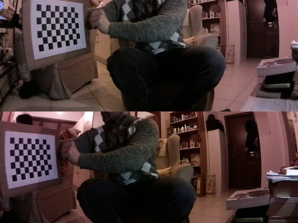
We can now open a live stream from the stereo camera by connecting to the UV4L streaming server with vlc (or with another suitable client) at the default URL http://raspberrypi:8080/stream/video.mjpeg (please replace “raspberrypi” with the proper hostname or IP address of your Raspberry Pi in your network).  The MJPEG stream should appear inside the vlc window; to extract a number of images (as .png files) press shift+s on the keyboard just as many times, i.e. whenever the chessboard is clearly on target and in a different pose. To improve the image quality, it’s possible to adjust some image settings “on-the-fly” (such as vertical and/or horizontal flip, brightness, contrast, etc…) through the web control panel at  the URL http://raspberrypi:8080/panel.

Below is one example (it’s noticeable the presence of radial distortion at the borders of the image):

Once we have acquired enough images, we can run the stereo calibration from command line as follows, for example:

$ ./stereo_calib --board-rows 9 --board-cols 6 --square-size 1 --num-imgs 20 --imgs-dir /path/to/imgs/ -e ".png" --top-bottom=1 --show-corners=1 --show-rectified=1 --output ./

In the above command, please pay attention to the correct path to the stereo images’ top-level directory (“/path/to/imgs/” in the example). square_size is the length of the side of the squares in the chessboard pattern. It can be measured in any units of length, for example in mm, or in “side units”, as above.  Keep in mind that depth values will be then expressed in the same unit of measure. Type –help in the command line for the list of all available options.

Below are the intermediate outputs of the calibration process that you can optionally enable, as in the above command line, to see and save them to disk (by pressing ‘s’ key in the window):

 

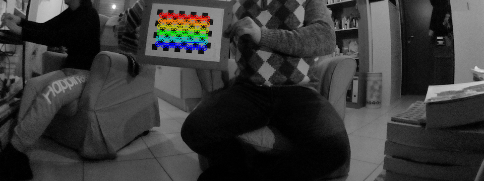
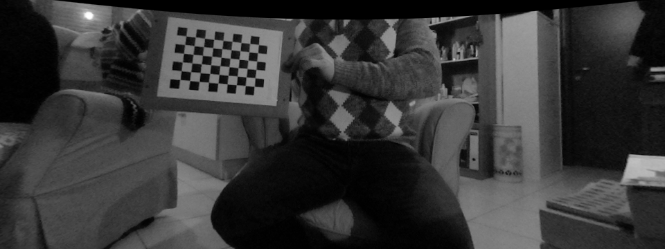
By default, the output of the command will be a stereo_calibration.xml file containing, among other things, the computed camera intrinsics, the lens distortion coefficients for each camera, the rototranslation matrix between the camera reference frames, the disparity-to-depth (re-projection) matrix, the image size.

IMPORTANT! stereo_calibration.xml file constitutes the fundamental input to UV4L for it to properly configure and run the stereo vision algorithms.

Stereo matching

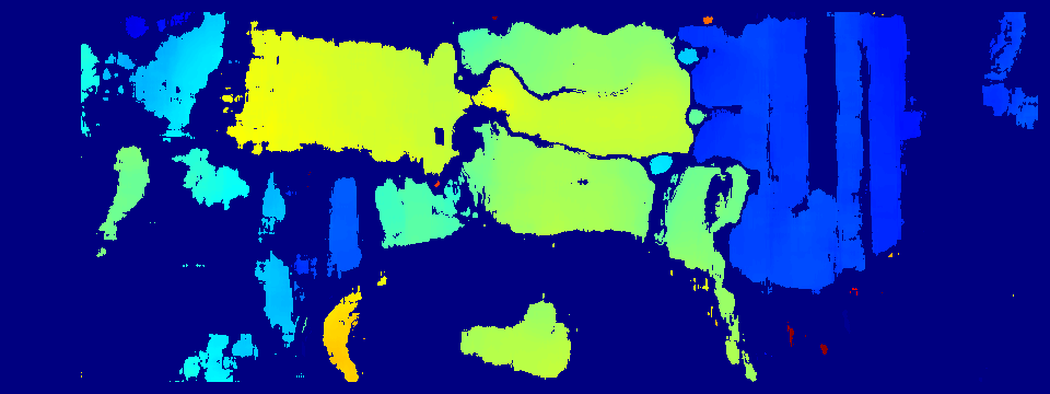
Stereo matching (or stereo correspondence) is about finding where a three-dimensional point appears in two different camera views. If the left and right images are rectified, correspondences can be found at the same row. In other words, for each feature pixel coordinate at (xl, y) in the left image a matching feature pixel (if any) in the right image must be found at coordinate (xr, y), whereby both pixels represent the same 3D point. Of course, this can be computed only in the visual area in which the camera views overlap. The difference d = xl – xr assigned with the pixel in the left image (typically) is called disparity (we assume the two principal points have zero disparity). Once we know the camera intrinsic parameters, the disparity can be triangulated to compute the depth measurement. The outputs of stereo matching applied to all the pixels in the image form a disparity map. The values in the disparity map can be mapped to a smooth color palette so that it is possible to display the map itself as an image giving the sense of depth of the scene (as an example, see the picture in the previous paragraph in the blue-yellow color map).

UV4L employs a stereo block-matching algorithm as the one found in OpenCV (cv::stereoBM) and exposes almost all the same options to fine-tune the algorithm for  specific use cases, especially those that define the disparity range that limit the search space for correspondences (which in turn defines the horopter in which 3D points belong to in the environment). This algorithm is not the most accurate, but it is faster than many others proposed in the literature and makes sense when it is going to be run by a general-purpose CPU.

The following options are not mandatory, but can be set in the UV4L configuration file (/etc/uv4l/uv4l-raspicam.conf), for example:

### dual camera & Stereo Vision options: 
stereo-matching-numdisp = 64
stereo-matching-blocksize = 29
stereo-matching-mindisp = 0
stereo-matching-uniquenessratio = 3
stereo-matching-texturethreshold = 5
stereo-matching-specklewinsize = 300
stereo-matching-specklerange = 9
# stereo-overlay-disparity-map = no

Interestingly enough, stereo-overlay-disparity-map in the above list allows to overlay the grey-level disparity map of the left view on the top of it in the full left-right-packed frame.

A short explanation of the meaning of each option can be found in the uv4l-raspicam driver manual or, alternatively, by typing the “uv4l –driver raspicam –driver-help” command:

$ man uv4l-driver
[...]
   --stereo-matching-numdisp arg (=0) 
disparity range to be considered for the stereo matching, must be multiple of 16, from 0 to 128

  --stereo-matching-blocksize arg (=21) 
block size used in the stereo matching algorithm, from 0 to 255 (odd)

   --stereo-matching-mindisp arg (=0) 
minimum value of disparity for the stereo matching algorithm, from -128 to 128

   --stereo-matching-uniquenessratio arg (=5) 
stereo matching post-filtering to remove a pixel with the best matching disparity if not unique enough, from 0 to 100

   --stereo-matching-texturethreshold arg (=10) 
filter out areas that don't have enough texture for reliable stereo matching, from 0 to 100 

   --stereo-matching-specklewinsize arg (=250) 
number of pixels below which a disparity blob is dismissed as speckle, from 0 to 1000

   --stereo-matching-specklerange arg (=2) 
how close in value disparities must be to be considered part of the same blob, from 0 to 31

   --stereo-overlay-disparity-map [=arg(=yes)] (=no) 
compute and overlay the dense disparity map onto the frame

Depth estimation

Depth estimation of detected objects in the left image derives from the previously computed disparity map straightforwardly. A rather simple approach is taken. For each (undistorted) object’s bounding box, a relatively small window area centered within the box is considered: each pixel in the window, for which a disparity has been found, is re-projected into the 3D world coordinates to obtain the corresponding depth. Then all the depths so found are averaged out and the result is labeled as the actual object’s depth. As you may understand, this approach works in so far as the pixels considered in the window really belong to the detected object. This may be an optimistic assumption in an uncontrolled environment (e.g. think of partially occluded detected objects). Future releases of this functionality might implement and offer other options to estimate depth, for example based on median or mode statistics.

Let’s put all together

First of all, it is important to recall that all the stereoscopic features in UV4L are implemented at driver level. In facts, uv4l-raspicam is a Video4Linux2-compliant driver. Therefore you access the input video device’s node /dev/videoX directly with any third-party V4L2-compliant application to capture single frames (at the moment, stereo vision is enabled when the video format in the device is set to YUV420 Planar only) .

That said, before making a point of all this tutorial with an example of live stream by means of the uv4l-server, we’ll have to make sure the minimum is properly enabled in the configuration file:

stereo-calibration-params = /path/to/my_stereo_calibration.xml
stereo-overlay-disparity-map = yes
stereo-object-depth-estimation = yes # object detection with TensorFlow must be also enabled 
tflite-model-file = /path/to/ssd_mobilenet_v2_face_quant_postprocess_edgetpu.tflite # or e.g. ssdlite_mobiledet_coco_qat_postprocess_320x320.edgetpu.tflite
tflite-overlay-model-output = yes

As usual, a short explanation of the above options can be found in the driver manual:

   --stereo-calibration-params arg 
path to the .xml file containing all the paramaters computed with stereo calibration

   --stereo-overlay-disparity-map [=arg(=yes)] (=no) 
compute and overlay the dense disparity map onto the frame 

   --stereo-object-depth-estimation [=arg(=yes)] (=no) 
enable depth estimation of detected objects (if object detection is enabled with TensorFlow)

   --tflite-model-file arg 
path to the .tflite SSD/CNN model file to be loaded into the EdgeTPU module.  Although the EdgeTPU accelerator is an optional device, if you want to make use of it, remember that the specified model must have been compiled for  this  device  specifically. The model must accept RGB input images with width multiple of 32 and height multiple of 16.

   --tflite-overlay-model-output [=arg(=yes)] (=no) 
draw model output onto the image: boundary boxes, confidence scores, class ids, etc... (might not be supported by all the video encodings). This option might slow down the framerate at high resolutions (up to 15%).

While stereo-calibration-params is mandatory, all the other options provide us with three possible use cases of the stereo vision features:

• live stream with no object depth estimation and with left view overlaid by disparity map computed on-the-fly: only stereo-overlay-disparity-map=yes is required;
• live stream with object depth estimation and without disparity map overlaid: stereo-object-depth-estimation=yes, stereo-overlay-disparity-map=no, tflite-overlay-model-output=yes, tflite-model-file must be set;
• live stream with both object depth estimation and disparity map shown: all the options mentioned in the previous cases must be enabled.

We can now restart the uv4l_raspicam service for the changes to take place:

$ sudo service uv4l_raspicam restart

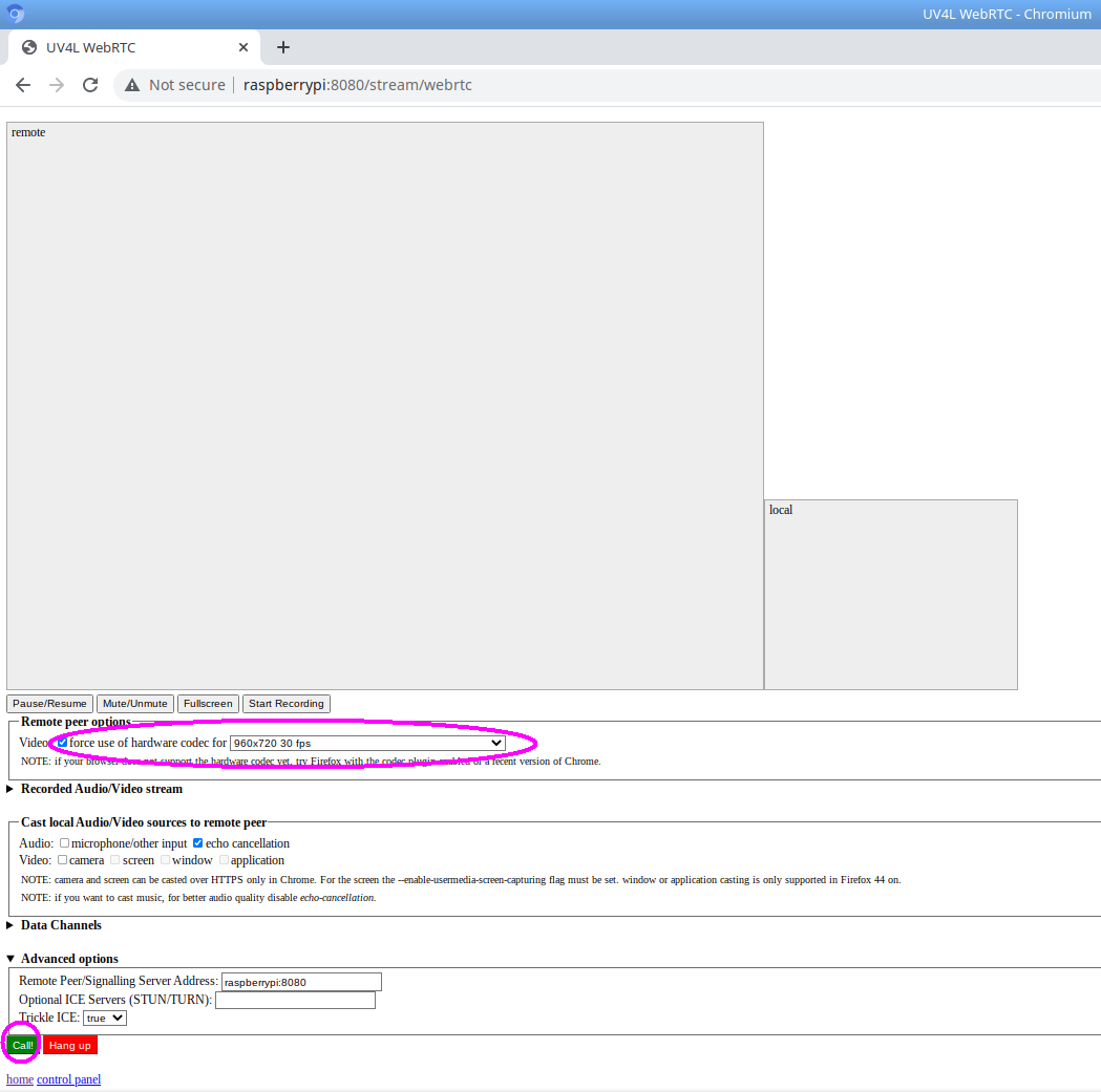
We can now open the WebRTC web page hosted on the Raspberry Pi (e.g. at the default URL http://raspberrypi:8080/stream/webrtc) where the UV4L streaming server is up and listening to, choose the same resolution for which we did the calibration (960×720 in this case), and finally click the call button to start the stream (see the circles in the picture below):

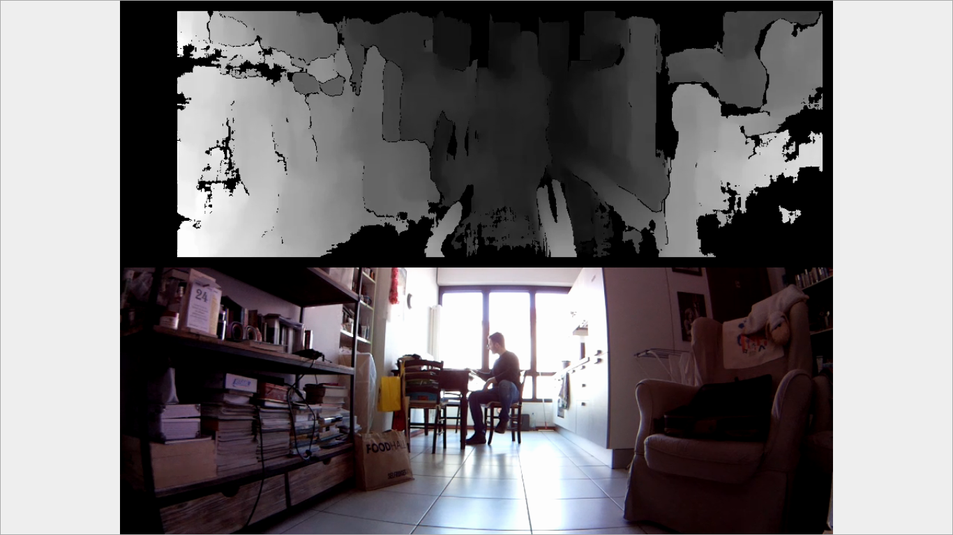
Below are some screenshots taken from the live stream shown in the browser window. You can clearly see the top of the frame overlaid by the disparity map associated with the left view and  the bottom half of the frame corresponding to the right view (originally distorted) . Both halves are synchronized.

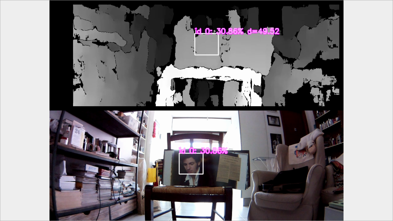
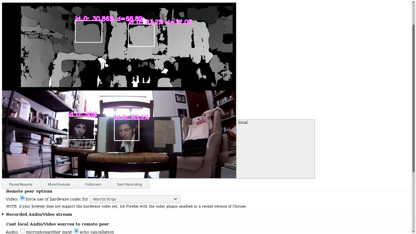
Whenever the object detection model recognizes objects in the frame (faces in this example), their respective bounding boxes will be overlaid onto the frame along with other related information such labels, classification scores and estimated depths.

Appendix. A naive stereo matching algorithm

As a proof of concept, what we present here is an implementation of a simple, non-optimized block-based stereo matching algorithm. It is not as accurate as the one mentioned in the previous sections. It is naive in the sense that it does not implement any filter to enhance the stereo images passed as input (e.g. the texture), or to prevent false matches. The algorithm just relies on the epipolar constraint of the rectified input images and employs the normalized cross correlation (NCC) as matching measure. The output of the algorithm is a disparity map associated with the reference (left) image.

More specifically, given a square block of size 2W+1 and a disparity range [dmin, dmax], at each pixel of coordinates (x, y) and intensity I(x,y) of the left image L, the NCC similarity function is computed among all pairs formed by the candidates belonging to the disparity range, as follows:

Then the disparity value to choose for the current pixel corresponds to the maximum of the NCC values computed on the pixels within the disparity range:

The overall computational complexity of the algorithm is O(width•height•(2W+1)²)•Drange) in the signal domain, which turns out to be rather slow without any further optimizations. Indeed, especially for architectures equipped with a FPU, the NCC can be implemented via Fast Fourier Transforms in the frequency domain, so as to scale the complexity down to O(width•height•log2(width•height)•Drange), independent of the block size.

Here is the source code of a program that takes two stereo images passed as inputs, converts them to grayscale and outputs, as an image, the disparity map computed by applying the NCC algorithm. The program makes use of two low-level helper functions of OpenCV, cv::matchTemplate() and cv::minMaxLoc(), which essentially carry out the two aforementioned equations. In particular, cv::matchTemplate() implements template matching via FFT and is called once per line, thus internally covering the whole range of disparities with a single function call.

After having built the program according to the instructions at the URL above, to get the list of available options, type the command below:

$ ./stereo_match --help
Program options: 
 -m [ --mindisp ] arg (=0)    minimum disparity 
 -n [ --numdisp ] arg (=64)   number of disparities 
 -b [ --blocksize ] arg (=21) odd block size 
 -l [ --left ] arg            path to the left image 
 -r [ --right ] arg           path to the right image 

Other options: 
 -h [ --help ]                print help screen and exit

The output of the program applied to the rectified stereo images shown in the previous section looks like this:

$ ./stereo_match --left left_rectified.png --right right_rectified.png --blocksize=17 --numdisp=64

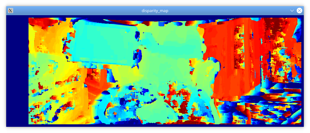
One advantage of the NCC is that the result is invariant to linear intensity changes of type Left=k•Right. Although in general this property makes this similarity function robust with respect to different lighting conditions between the left and right captures, this is usually not a problem in stereo vision, because both the images are captured “at the same time”, thus under the assumption of same lighting conditions (and also under the implicit assumption of Labertian surfaces present in the scene). This is one reason why, in this context, it’s preferable to just rely on a faster matching measure such as SAD, without having to worry about  robustness in practice.

A first attempt to clean up the disparity map from noise would be to apply a median filter and possibly a bilateral filter afterwards, which can smooth the disparity map by preserving edges, but this is left an exercise to the reader.